SHRUG Quickstart⚓︎
Welcome to the SHRUG quickstart tutorial. This will be your entry point to accessing data on the SHRUG platform. This tutorial is primarily written for Stata and Python users.
Data available for download here
Example 1⚓︎
Let's take a look at some population census data. Download the Population Census Abstract files for 1991 and 2011, alongside the Economic Census modules for 1990 and 2013. The example below assumes the files are saved to your ~/Desktop, but you can put them anywhere you like. Let's explore some trends in employment over the past three decades:
/******************************************/
/* Set globals to where the data is saved */
/******************************************/
global shrug ~/Desktop
/* Let's merge population census data at the village-town level across 1991-2011 */
use $shrug/pc91_pca_clean_shrid, clear
qui merge 1:1 shrid2 using $shrug/pc01_pca_clean_shrid, keep(match) nogen
qui merge 1:1 shrid2 using $shrug/pc11_pca_clean_shrid, keep(match) nogen
/* Now bring in employment from the economic census */
qui merge 1:1 shrid2 using $shrug/ec90_shrid, keep(match) nogen
qui merge 1:1 shrid2 using $shrug/ec13_shrid, keep(match) nogen
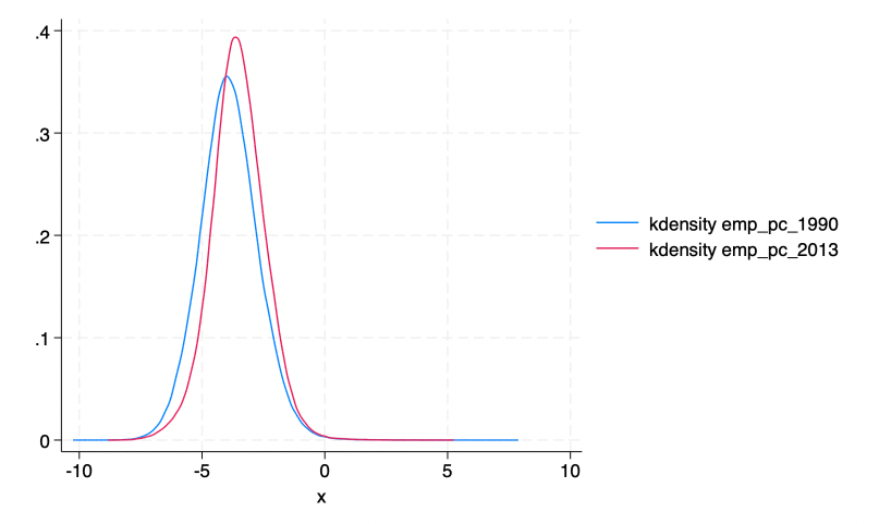
/* Construct log employment per capita */
gen emp_pc_2013 = log(ec13_emp_all / pc11_pca_tot_p)
gen emp_pc_1990 = log(ec90_emp_all / pc91_pca_tot_p)
/* Next, graph the distributions of employment for a rudimentary comparison */
twoway (kdensity emp_pc_1990) (kdensity emp_pc_2013)
# import pandas
import pandas as pd

# load shrug population census data for all 3 rounds
shrug_pc91 = pd.read_stata("shrug_pc91.dta")
shrug_pc01 = pd.read_stata("shrug_pc01.dta")
shrug_pc11 = pd.read_stata("shrug_pc11.dta")

# merge data from all rounds
shrug_merged = shrug_pc91.merge(shrug_pc01, on = "shrid", how = "inner")
shrug_merged = shrug_merged.merge(shrug_pc11, on = "shrid", how = "inner")

# aggregate data to national totals
shrug_total = shrug_merged[['pc91_pca_tot_p', 'pc01_pca_tot_p', 'pc11_pca_tot_p', 'pc91_pca_tot_p_u', 'pc01_pca_tot_p_u', 'pc11_pca_tot_p_u']].agg(['sum'])

# calculate percentage of urban population in each decade
shrug_total["urban_91"] = shrug_total["pc91_pca_tot_p_u"] / shrug_total["pc91_pca_tot_p"]
shrug_total["urban_01"] = shrug_total["pc01_pca_tot_p_u"] / shrug_total["pc01_pca_tot_p"]
shrug_total["urban_11"] = shrug_total["pc11_pca_tot_p_u"] / shrug_total["pc11_pca_tot_p"]

# plot bar graph of urbanization rate
shrug_total[["urban_91", "urban_01", "urban_11"]].plot(kind = "bar")
Example 2⚓︎
Example 2 requires the 2011 Population Census Abstract as well.
Motivating hypothesis: In economics, it is commonly believed that during the demographic transition, families have fewer children and those children get more education. This is sometimes called the "quantity-quality" tradeoff.
Translating into our data: Between 1991 and 2011, average number of family members fell as literacy rates rose.
/* First, merge in the 2001 PC data. */
merge 1:1 shrid2 using $shrug/pc01_pca_clean_shrid, keep(match) nogen
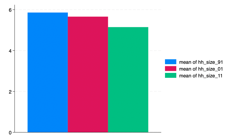
/* Let's calculate the average number of family members per household */
gen hh_size_91 = pc91_pca_tot_p/pc91_pca_no_hh
gen hh_size_01 = pc01_pca_tot_p/pc01_pca_no_hh
gen hh_size_11 = pc11_pca_tot_p/pc11_pca_no_hh
/* let's check the values of household size for outliers */
sum hh_size_*, detail
/* Some households are 700 people. Assume that average household size does not exceed 10 */
replace hh_size_91 = . if hh_size_91 >= 10
replace hh_size_01 = . if hh_size_01 >= 10
replace hh_size_11 = . if hh_size_11 >= 10
/* let's visualize household size across 3 time periods */
graph bar (mean) hh_size_91 hh_size_01 hh_size_11
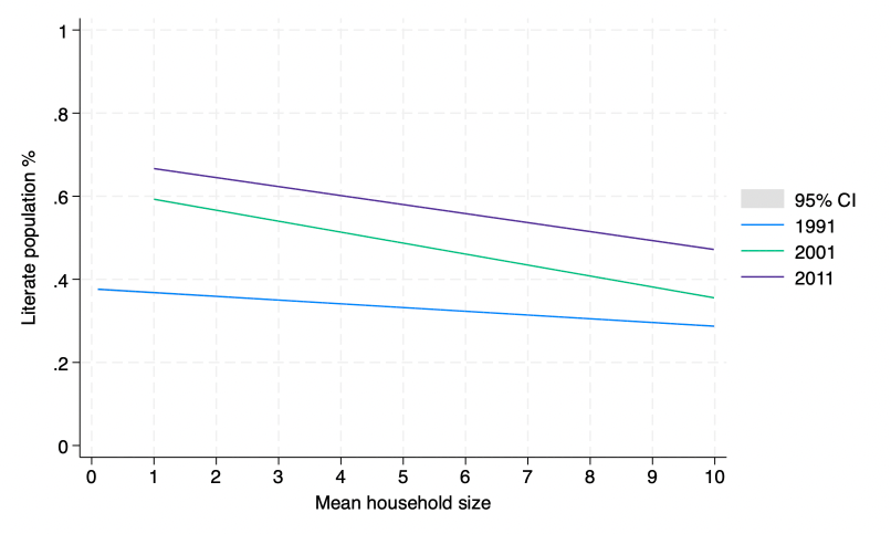
/* let's create literacy rates */
gen lit_91 = pc91_pca_p_lit/pc91_pca_tot_p
gen lit_01 = pc01_pca_p_lit/pc01_pca_tot_p
gen lit_11 = pc11_pca_p_lit/pc11_pca_tot_p

twoway (lfitci lit_91 hh_size_91) (lfitci lit_01 hh_size_01) ///
(lfitci lit_11 hh_size_11, legend(label(2 "1991") label(3 "2001") label(4 "2011")) ///
 ytitle("Literate population %") xtitle("Mean household size") ///
 ylabel(0 (0.2) 1) xlabel(0 (1) 10))
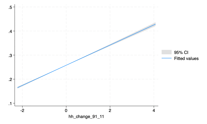
/* let's calculate the change in average household size in each village from 1991 to 2011 */
gen hh_change_91_11 = ln(hh_size_11) - ln(hh_size_91)

/* let's calc the average change in literacy rate between 1991 and 2011 */
gen lit_91_11 = lit_11 - lit_91

/* Graph the relationship */
twoway (lfitci lit_91_11 hh_change_91_11)